
An Introduction
Creating hundreds or thousands of solutions for a problem might sometimes sound like an overkill but what if a method inherently creates thousands of diverse solutions while looking for the best performing ones on the way? Not only could we find the one solution we might have been looking for all along, but we find hundreds of solutions that solve a problem in different ways.
Imagine using this for creating different Reinforcement Learning Agents, Robotics Controllers, or even to create different neural networks while each solution is the best it could be for its specific behaviour. This is exactly where Quality-Diversity algorithms come into play and this blog will try to introduce you to them.
To start with Quality-Diversity Algorithms, it might be good to draw similarities with nature and evolution. Personally, I tend to understand things better when I have something real to compare it with and in this case it’s our evolution. In no case is evolution the only use-case for Quality-Diversity algorithms but it provides a good motivation on why it works well. If you would like to learn directly about the algorithms (or feel comfortable with evolutionary algorithms) then feel free to skip to the part about Behavioural Descriptors as they play a key role in this kind of algorithms.
Evolution and Humans
Interestingly, nature has created intelligence in many different ways. Some of the intelligence we know well (but still not fully understand) is our own human intelligence. Many millions of years ago, the first living cells formed themselves through a combination of unplanned events. None of these processes were directly planned by somebody or something and still, here we are. The unfolding of many “random” steps have led to many different organisms that have each remarkable qualities.
Just when thinking about this, I am in full admiration of what nature and evolution have brought to life.
The idea I want to get at behind this process is that there was no goal or idea behind any of these processes. Diversity is the key to this process since evolution uses this as a steppingstone to find new organisms or to improve existing ones. Darwinism for example states that there is a survival of the fittest. The mutations of the genes of each animal will determine whether or not they are well enough adapted to the environment and its constrains.
Now what if we would use this idea and apply it to Optimization? This idea of creating a lot of parallel processes, which enable different solutions, is very powerful and has already been applied to different problems. Quality-Diversity algorithms are using this idea as well and they have been very successful at optimizing various problems ranging from robotics to games. While I will try to introduce you to Quality-Diversity (QD) algorithms in the next sections, I think it will always be helpful to think about this evolutionary process that created us humans.
Evolution applied to Optimization Problems
A lot of researchers have already tried (and successfully so) to apply this principle of evolution to optimization problems. Luckily, there is a great guide by David Ha2 about different evolution strategies that covers all the basic knowledge that is needed to understand how evolution strategies can be used to optimize functions. The nice thing about using evolutionary algorithms is that usually we don’t require a gradient to get to the best solution, but we rather let evolutionary pressure do its thing. This allows us to do black-box optimization for functions where it is impossible or very difficult to calculate a gradient and apply methods like stochastic-gradient descent. In evolution we often talk about the terms genotype and phenotype, which can be quite confusing at some points and I will do my best to describe this in the best possible way.
As a short recap, we can say that a generic evolutionary algorithm incorporates 6 steps:
- Create a population of individuals (random generation): These individuals can be represented for example by vectors of real numbers that represent a part of the solution we need (genotype) which can be the parameters of a robot/agent. The individuals defined by these vectors themselves are called the phenotype (i.e., the expression of the genotype).
- We iterate through each of these individuals and calculate their fitness function (i.e., how good they solve our task or approximate our function)
- We select the best individuals with respect to this fitness function (Parents)
- New individuals are created by copying the selected individuals and mutating them (we mutate the genotype) and/or by doing a cross-over of two individuals to create one new one (Offspring)
- We add the offspring to our population and eliminate the least fit individuals in the population during the process. We then go back to Step 3. and execute all the steps until a limit is reached (i.e., fixed computational budget, or threshold in the fitness function)
- When we are done, we will have a population of high performing solutions
Usually, you want to optimize one function and in many cases this function describes a fitness to a certain goal. This can for example be a minimum of a function (e.g., a loss function that describes the error that we make and we need to minimize that error) and we could say this is the quality of the solution.
I am introducing the generic concept of evolution algorithms so that you can draw parallels between the two approaches. You can see that the evolutionary algorithm can optimize the fitness function, and this is what it has been designed for.
However, Quality-Diversity goes further and introduces a second aspect to the optimization of a function, namely the diversity of solutions. This is a very important notion since it allows us to discover a variety of solutions that all have different characteristics (in terms of behaviour as you will discover soon). Keeping a range of very good and diverse solutions can be very helpful for a variety of applications. In robotics for example, having a lot of solutions allows us to be much more adaptable to our environment since we can switch between the known solutions depending on the behaviour that we need.
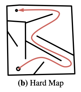
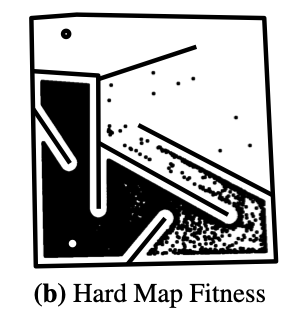
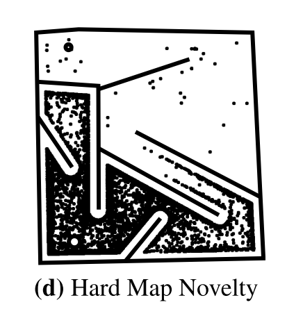
Let’s have a look at the HardMaze example that has been presented by Lehman, J., & Stanley, K. O. in 20113(images have been taken from the paper by Wooley B. G. & Stanley, K. O.4 ). The goal is to move the big circle (a mobile robot) at the bottom to the small circle on the top. In this case, the fitness function is the direct distance between the robot and the small circle. If we would try to optimize only for this fitness function, we would quickly be stuck in a local minimum and never reach the point as you can see on the “Hard Map Fitness” picture on the right. All the solutions focus on the upper left dead end of the maze since the distance there is very small. However, we are not able to solve the maze (i.e., no solution reaches the little, small circle on the top. To overcome this, we want to focus not only on optimizing on performance but also on the diversity of solutions. More on diversity in the next sections and it will also show you how we can solve this maze differently than simply using a quality metric.
What about the diversity of the solutions?
Behavioural Descriptors
Let us get there in a second but first let’s see what we need to define diversity in our solution. Every solution we create in this evolutionary process will be an individual with a specific behaviour. We define a behaviour descriptor, a set of features to characterise the different types of solutions generated by the algorithm. This behaviour could be a very easy definition such as the end xy-coordinates of a walking robot or the duration of ground contact that each leg of a hexapod has during its walk. The behaviour of a solution is usually defined by an engineer or researcher who wants to identify different solutions in terms of behaviour (not only in terms of fitness). And this is what we call the diversity aspect of the solutions, i.e., having a lot of solutions in our population that are as diverse as possible, meaning that they all have different behaviours (even if the fitness might be worse).
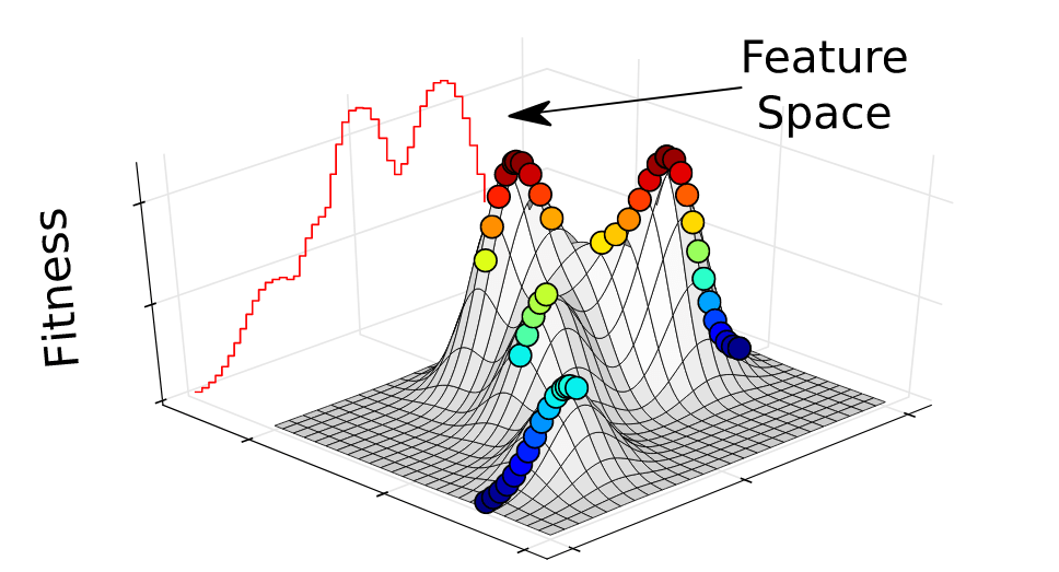
 The Behavioural Descriptors can easily be mapped to a map as you can see in the graphs below. Remember, that the only purpose of these descriptors is to map a given solution (with all its parameters) to a specific behaviour and save it there.
One example of a Behavioural Descriptor Map can be seen in the figure below. This map shows the x and y gripper coordinate that an 8 Degree of Freedom (DoF) arm can reach. The arm itself is similar to the one shown on the right side where each arm link is connected by a rotor that can turn to any angle we need.
We see that the shape of the Behavioural Descriptor Space (BD) is round, which makes sense if we think about all the possible points the arm on the right could reach potentially. Each point in the map represents one solution that can reach this point; hence it shows us the diversity of the solutions. The colours here show what the fitness function is, meaning that for each solution, we can have another fitness value (the higher, the better). In this case the fitness function is the variance between all the angles in robot arm. As you might wonder, the map I show you below is not symmetrical, and this is due to the task setup (specification) and the orientation of the first link.
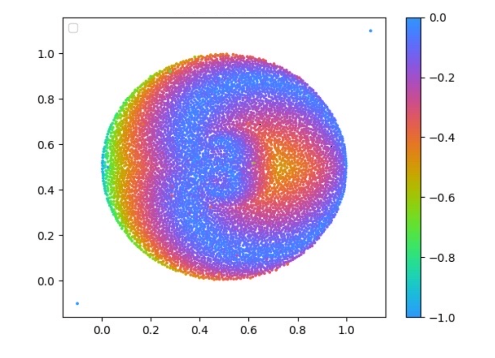
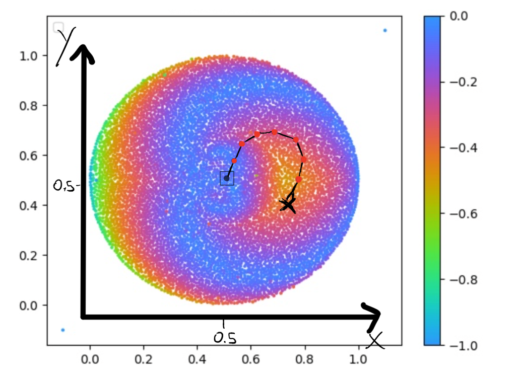
This means if we look at this map, we could select any point and get the parameters for this solution (e.g. the parameters for the model, here the rotor angles). You can see that when selecting a point on the right picture, we have our robot arm in the configuration so that it can reach this point.
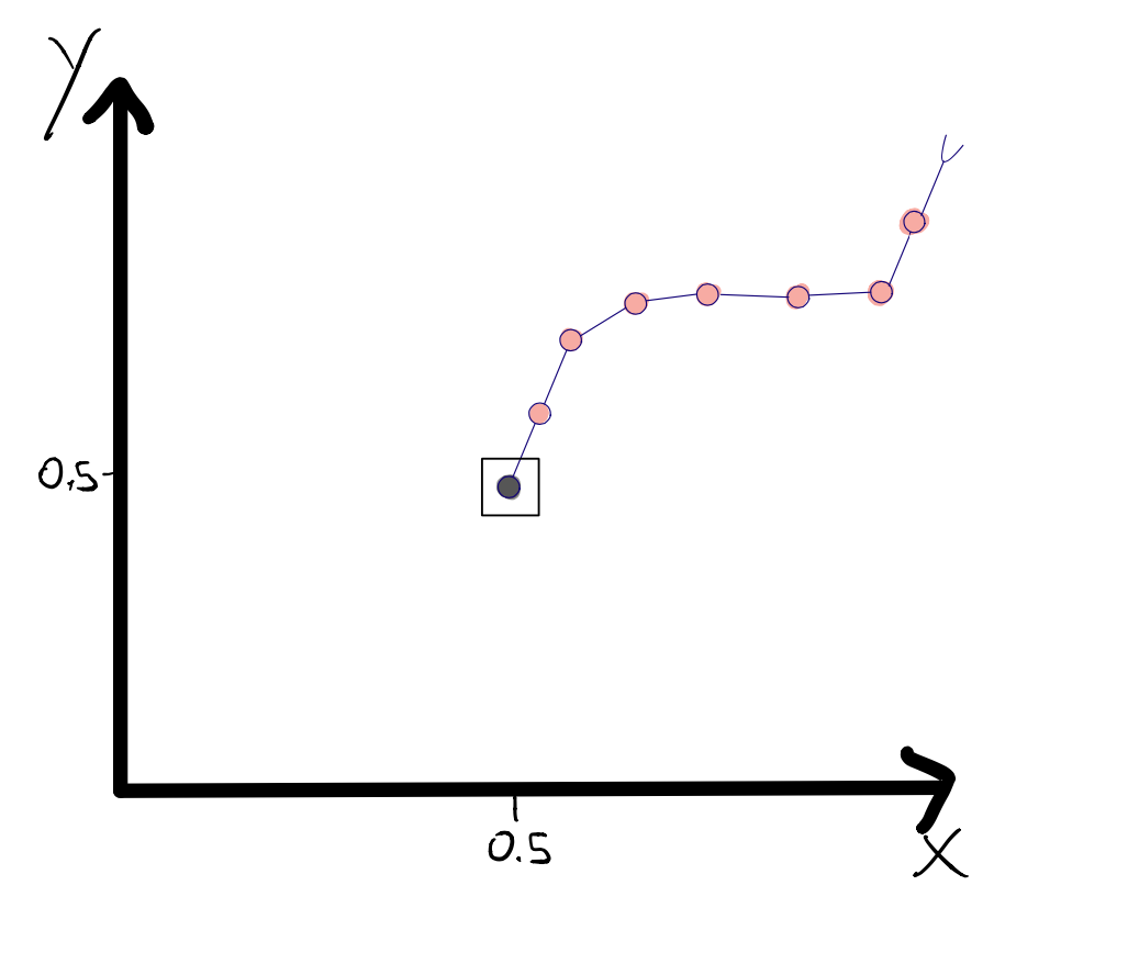
Another fun example is the one of an Hexapod that walks into many different directions like the one we can find in this paper by Antoine Cully et al.5. You can see both the end x and y coordinates as well. The arrows here, show us what the final orientation of the robot is.
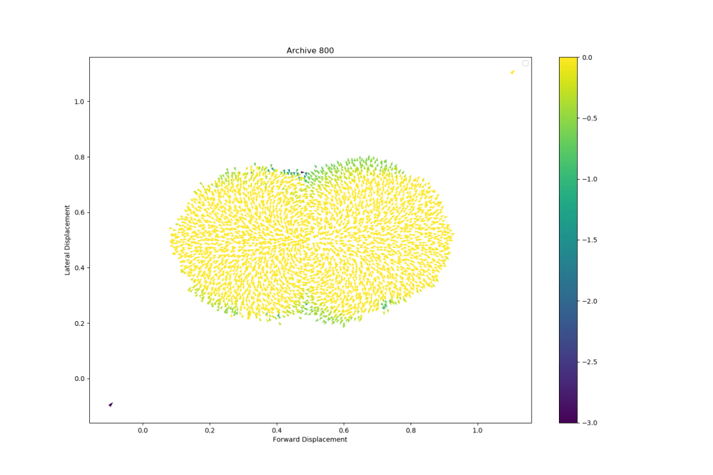
As you can see, the algorithms can create thousands of high-performing solutions that each have another behaviour. Here the behaviour descriptor in the map was defining in how many directions the hexapod could walk by observing the lateral and forward displacement at the end of the walk. The robot started at point (0.5,0.5) on this map so anything below 0.5 and above 0.5 defines two different directions. We could now select different solutions and run our robot with them, meaning that we can control our robot to reach thousands of different positions with a high performing controller (due to the good quality of each solution).
Now you should have a good understanding of what a Behavioural Descriptor is and that it could be defined many different ways!
These two examples are the outcomes of Quality-Diversity Algorithms and this is exactly what the next section will be about. If you still followed up until this point, then the next few sections will be really easy to understand!
These examples show us why we would want to use Quality-Diversity algorithms instead of other optimisation algorithms. A few points include:
- We can keep not only one single (good) solution, but we can create a lot (thousands!) of unique and diverse solutions and choose between them (or use them together)
- We can illuminate a behaviour space, meaning that we can discover a lot of different behaviours that are possible which is usually not trivial. Imagine discovering behaviours that you didn’t think off before which could lead to creativity boosts in your solutions
- We can use weak solutions as “steppingstones” that allow us to jump over local minima and find the global minimum
- Optimizing both for Diversity and Quality can be applied to a lot of different domains and ideas and is not only restricted to Evolution or Robotics for example
Maybe it would be good to really introduce the notion of Behavioural Descriptor in the previous paragraph, just saying clearly that this is how we call them.
People who are not used to this task might ask why the map is not symmetrical and thus think they did not get something about the algorithm when it is just a specification of the task (I get the question every time) . I don’t know if you can really do anything to prevent this, but maybe mentioning it would help?
Maybe this is not obvious to visualise for new QD users. Would it be good to have a little figure that makes the link between your two last figures? For instance, a figure decomposed in two:
(1) on the left, there would be the archive itself with a black cross somewhere, (2) on the right, there would be an image of the corresponding behaviour where we see the arm.
I have just noticed that the words “behavioural descriptor” are never used in the next sections, especially for the Hexapod task, where it is not explained in which sense the behaviours are different.
Quality-Diversity and MAP-Elites
Combining Novelty Search with Interactive Evolution4
As explained above, Quality-Diversity or QD from now on, is this family of algorithms that goes and creates thousands of diverse, yet high performing solutions. This is not only a good thing to plot nice, coloured graphs but the fact that we keep a diverse population of solutions allows us to find steppingstones in our solution search that we wouldn’t find otherwise. Coming back to our example of the HardMaze in the upper left picture, where the small circle on the top is the objective and the larger circle on the bottom is the robot. As a reminder, the goal is to reach the small circle. If we only look to minimize the fitness function (i.e., the distance to the circle), it can be shown that the algorithm will never solve the maze but rather stay in the local optimum (upper middle picture). Novelty Search3 (only looking for diversity, not quality) on the other hand, is able to find solutions that are much closer to the small circle even though it wasn’t even guided through a fitness function.
This shows that just looking for novelty allows to find steppingstones (i.e., individuals that are mutated) that can lead to high performing solutions, even though it might not be the most direct path. Quality-Diversity is trying to leverage this aspect of finding very diverse solutions while keeping only the best ones for each diverse behaviour (as defined by the behaviour descriptor). If two solutions are identical in terms of behaviour, then only the best one will survive. This idea is very powerful since it will allow us to get thousands of high performing solutions that are the best ones (elites) among their behaviour.
The easiest way to explain it, is by walking through one specific QD-Algorithm called MAP-Elites (you can read more about it in the paper “Illuminating Search Spaces by Mapping Elites” from Jean-Baptiste Mouret and Jeff Clune6).
Multi-dimensional Archive of Phenotypic Elites (or simply MAP-Elites)
While we go through this, it might be useful to keep both pictures of the Behavioural Descriptors in mind since it will combine all the above-mentioned points!
MAP-Elites specifically takes the inspiration from evolution and tries to find solutions by mutating a set of solutions and producing offspring. This is only one form of QD, and it allows us to showcase how powerful QD can be. You will see that MAP-Elites is a simple, yet very effective approach to do QD optimization.
MAP-Elites allows us to keep track of fitness and diversity via the structured archive (here an n-dimensional grid. For MAP-Elites, the archive and the individuals in it are our final solution.
To better understand what is going on, we could have a look at the pseudo-code of the algorithm and since the algorithm itself is not too complicated, it can be replicated very quickly and applied to any field:
Def Map_Elites(){
P <- N-Dimensional Map for performance of the solution
M <- N-Dimensional Map for the parameters of the solution
K <- Number of Iterations
For iter=1 -> K do {
 If iter==1: Create random Population and fill into P
 Else{
  #Select randomly individuals from P
  Parents <- Select_Randomly(P)
  #Mutate them
  Offspring <- random_mutation(Parents)
  }

 For Individual in Offspring do{
   # We evaluate the solution
   (Descriptor,Fitness) <- Evaluate(Individual)

    If M[Descriptor]==Empty or P[Descriptor]<Fitness{
     # We store our solution into the Map
     M.add([Descriptor,Individual])
     # at the Index defined by the BD
     P.add([Descriptor,Fitness])
     }
   }
  }
Return (P,M) # with the solutions
}
We can see that the algorithm is trying to keep diverse solutions by mapping them to a grid or map and only replaces a solution if there is a more performing solution for this exact position on the grid. The map that is returned is the one we saw previously!
Here above is one nice example of such a map for a hexapod from the Paper “Robots that can adapt like animals”7. The behaviour descriptors we can see in this map is the contact duration between the legs and the ground. This specific paper used this map to help the robot adapt to different situations (e.g., broken leg) once it has been deployed. You could imagine that the robot learned at some point to only walk with 5 legs instead of 6 and the idea is to find this behaviour with another algorithm and apply it to the broken robot so that it can walk straight again. This aspect of adaptive robots is very promising and can lead to very exciting applications in the industry.
Besides MAP-Elites there are other QD algorithms8, such as for example Novelty Search with Local Competition9, which is using an unstructured archive where instead of cells with a fixed size we add solutions to the archive if they are novel enough (based on the k-means distance to other solutions). In addition to an archive, the NSLC algorithm uses a population since the end result of the algorithm is not the archive but rather the population. If you want to learn more about this method, the paper is directly linked with the name so you should be able to find it easily.
Start Using QD yourself!
You certainly ask yourself, ok this sounds nice but how can I start experimenting with these sorts of algorithms. Do not worry, we got you covered! Luckily there are some nice libraries out there that can help you use QD with good tutorials.
Python:
For Python lovers, there are three libraries that can be used:
- PyMap_Elites: https://github.com/resibots/pymap_elites
A very clean and neat implementation that is easy to understand and allows for nice extensions
This framework is a little more advanced and allows you to have more flavours to your QD algorithm
- PyRibs: https://pyribs.org
PyRibs is a new library that has very nice tutorials and is also a framework that allows you to do more specific things within QD. A nice example is the one that we showed above where we use a robotic arm to reach every position in the space. You can even open the tutorial in a colab notebook.
C++:
For the performance lovers, there is also a very powerful framework that allows you to run Evolutionary Computations in C++:
- Sferes2: https://github.com/sferes2/sferes2
This framework is very flexible and allows you to do a lot of things while being very efficient. Since this library is a powerful framework to run any Evolutionary Algorithm, I suggest having a look at the ‘QD’ branch since it allows you to do all the QD stuff we just talked about and has most methods already implemented so that you can have a go at it.
I hope this little tutorial helped you to get some insights into QD and MAP-Elites and it further sparked your interests to use this in your research or your industry!
This blog is rather a light introduction to the topic and is meant for everybody who wants to learn more about QD and the principles behind it. If you are interested in more specific applications, there are already a good number of papers out there that use QD for Games, Reinforcement Learning, Robotics and so on. It’s a really exciting community that is quickly growing and you best start on the website https://quality-diversity.github.io/. This webpage is great since it contains tutorials from experts as well as a full collection of papers on this topic.
Finally, thanks to Antoine Cully, Bryan Lim, Manon Flageat and Luca Grillotti from the Adaptive & Intelligent Robotics Lab for their valuable comments.
References
1. Chatzilygeroudis, K., Cully, A., Vassiliades, V. & Mouret, J.-B. Quality-Diversity Optimization: a novel branch of stochastic optimization. arXiv (2020).
2. Ha, D. A Visual Guide to Evolution Strategies. (2017).
3. Lehman, J. & Stanley, K. O. Abandoning objectives: Evolution through the search for novelty alone. Evol. Comput. 19, 189–222 (2011).
4. Woolley, B. G. & Stanley, K. O. A Novel Human-Computer Collaboration: Combining Novelty Search with Interactive Evolution. doi:10.1145/2576768.2598353.
5. Cully, A. & Mouret, J.-B. Behavioral Repertoire Learning in Robotics.
6. Mouret, J.-B. & Clune, J. Illuminating search spaces by mapping elites. (2015).
7. Cully, A., Clune, J., Tarapore, D. & Mouret, J.-B. Robots that can adapt like animals. doi:10.1038/nature14422.
8. Cully, A. & Demiris, Y. Quality and Diversity Optimization: A Unifying Modular Framework. IEEE Trans. Evol. Comput. 22, 245–259 (2018).
9. Lehman, J. & Stanley, K. O. Evolving a Diversity of Creatures through Novelty Search and Local Competition. (2011).

Thanks for your article. Do you have a suggestion for a paper or library satisfying these conditions:
* The topology evolves, like NEAT
* The nodes in the topology can be functions that don’t necessarily have the same argument types or number of arguments (arity). NEAT seems to rely on aggregations and activation functions but can’t treat nodes as generic functions. For example, Karl Sims’ paper (https://www.karlsims.com/papers/InteractiveEvolutionVisualComputer93.pdf) uses LISP and the LISP functions have different argument types/arity.
* It’s graph-like, not tree-like, so the output of a node can be reused as the input to several other nodes.
LikeLike